Polish, Device, and Scale
After any stochastic driver you run a deterministic “last mile”. The same polish component also works as a pure multi-start method (QMC or shifted-QMC). The device path (NumPy or CuPy) and the batched ensemble runner execute the identical transition kernel; only the array namespace and leading batch axis change.
Reference
DeviceHistory / EnsembleHistory, run_device, run_ensemble, the projected-gradient Armijo backtrack, and the low-discrepancy screening live in python/anneal/device.py (thin wrappers) and the Rust runner / local_polish. The “same kernel” claim is the algebra in action: the five-component object is what gets executed on the device.
Prerequisites
For polish variants a gradient is required. Device examples work with plain NumPy; GPU examples need CuPy on a CUDA machine.
Step 1: Polish after a stochastic run (projected Armijo)
import numpy as np
from anneal import Boltzmann, run, polish

def rastrigin(x):
    return 10.0 * len(x) + np.sum(x*x - 10.0 * np.cos(2.0 * np.pi * x))

def grad_rastrigin(x):
    return 2.0 * x + 20.0 * np.pi * np.sin(2.0 * np.pi * x)

low = np.full(5, -5.0)
high = np.full(5, 5.0)

hist = run(rastrigin, low, high, Boltzmann(t_init=8.0, sigma=1.5),
           n_epochs=15, steps_per_epoch=60, seed=3)
x0 = hist.best_pos

refined = polish(rastrigin, grad_rastrigin, low, high, x0,
                 max_fevals=300, step0=0.5, grad_tol=1e-8)
print("After polish best:", refined["best_pos"], refined["best_val"])
The polish performs backtracking projected gradient steps with the Armijo sufficient-decrease test inside the box.
Step 2: QMC / shifted-QMC polish as a standalone multi-start
Screen low-discrepancy points (or shifted replicates) and send the best k of them to polish.
from anneal import qmc_polish, shifted_qmc_polish

out_q = qmc_polish(rastrigin, grad_rastrigin, low, high,
                   n_starts=128, max_fevals_per_start=30,
                   seed=0, top_k=4)
print("QMC polish best:", out_q["best_val"])

out_s = shifted_qmc_polish(rastrigin, grad_rastrigin, low, high,
                           n_starts=64, max_fevals_per_start=30,
                           seed=0, n_replicates=2, top_k=1)
print("Shifted-QMC polish best:", out_s["best_val"])
Step 3: Device and ensemble (identical kernel)
from anneal import run_device, run_ensemble

# Host (NumPy) single chain
h1 = run_device(rastrigin, low, high, Boltzmann(t_init=10.0, sigma=1.0),
                n_epochs=8, steps_per_epoch=40, seed=9)
print("Device (host) best:", h1.best_val)

# Batched ensemble (same kernel, extra batch axis)
h2 = run_ensemble(rastrigin, low, high, Boltzmann(t_init=10.0, sigma=1.0),
                  n_chains=256, n_epochs=4, steps_per_epoch=25, seed=9)
print("Ensemble global best:", h2.global_best_val)
Replace low/high with CuPy arrays and the kernels run on GPU with zero Python overhead inside the loop. The returned DeviceHistory / EnsembleHistory keep every field on the original device and expose DLPack.
Why this works (reuse)
run_device and run_ensemble are thin shims around the same Rust runner that run uses.
The transition kernel they execute is the five-component Sampler object (Obj + Cool + Neigh + Move + Accept) that the presets and advanced drivers construct.
The batched device path only adds a leading axis to state and to the objective/gradient evaluations; the acceptance logic, cooling schedule, and proposal generation use the same code paths.
Consequently the noise-aware compensated Accept, the GLE Move, and the rank-1 independence Move are available on GPU and in large ensembles when the same slots are selected.
QMC polish is likewise a pure filling of the same slots (a deterministic Cool that goes to zero, a Move that is projected gradient, an Accept that is Armijo). The polish variants share the same Armijo logic and low-discrepancy generator.
Figures and scale experiments
GPU vs host scaling curves, ensemble saturation plots, and the CUTEst performance profiles that include the polish post-processing step are produced by experiments/scripts/render_plots.py and the cutest-full pixi tasks.
All numbers in the paper were regenerated from the identical sources (see used-by page).